Chapter 6 Overfitting
Following our exploration of the bias-variance tradeoff, in this chapter we explore the equally crucial concept of overfitting in machine learning.
Through the compelling stories of Baron’s travel planning and Jennifer’s exam preparation, we’ll uncover how overfitting manifests in both everyday scenarios and complex algorithms, revealing its impact on decision-making and model accuracy. Let’s extend Baron’s story from the previous chapter, which not only illustrates the bias-variance tradeoff but also seamlessly incorporates the concept of overfitting, providing a deeper understanding of its implications.
As we mentioned at the beginning of previous chapter, Baron initially developed a routine to leave his house around 7:00 AM, with a 30-minute window on either side to catch his bi=weekly flights. This approach, while seemingly flexible, had high variance. It is like a machine learning model that is not sufficiently trained or fine-tuned – it has a broad range of responses (leaving times from his home) but lacks precision (cathing flights).
Realizing the issue with his initial strategy, Baron decides to analyze past data more closely. He starts noting down the exact traffic conditions, weather patterns, and personal preparation times for each day of his travel. Based on this detailed analysis, he creates a very specific and complex routine, factoring in all these variables to predict the optimal departure time. This new strategy is akin to an overfitted model in machine learning – it is overly complex and tailored to past data, potentially capturing random error (like a one-time traffic jam or an unusual personal delay) rather than the overarching trend.
Initially, Baron’s new strategy seems to work perfectly, as he catches his flights consistently. However, on a day with unexpected conditions (not previously encountered in his data, like a new road closure), his overly complex routine fails him, and he continue to miss some of his flights. This is similar to an overfitted model performing well on training data but poorly on new, unseen data.
Baron realizes that his overfitted strategy is not sustainable. He then revises his approach, aiming to leave around 7:05 AM with only a 10-minute window. This strategy introduces a slight bias (always leaving a bit later than the original 7:00 AM plan) but significantly reduces variance. It is like a well-balanced machine learning model that has been trained to generalize well, rather than just perform on specific past data.
With this balanced approach, Baron consistently catches his flights, demonstrating that a balance between bias and variance can lead to more effective real-world results. His experience underscores the importance of not overcomplicating models (or plans) based on past data, as real-world conditions often present new, unforeseen challenges. This balance is crucial in machine learning to create models that perform well both on historical data and in new, unpredictable situations.
After discussing Baron’s experience, let’s shift to another example that deepens our grasp on overfitting. We now turn to Jennifer, a student facing challenges in her study methods for a history exam. Her story, paralleling Baron’s, can illustrate the concept of overfitting in everyday situations and in machine learning models.
Jennifer gathers an array of study materials, including textbooks, class notes, and online resources. She compiles detailed notes on all the topics that might be covered in the exam (Data Collection). She initially tries to get a general understanding of all historical events and themes, but soon realizes it is too much to handle. As she studies, Jennifer notices that certain events and dates are emphasized more in her materials (Pattern Recognition). Then, Jennifer forms a hypothesis that the exam will primarily consist of questions about these specific events and dates she has identified as important (Making Predictions).
Jennifer faces a dilemma. She can either maintain a broad focus on history, which would result in a high bias but low variance in her study approach, potentially causing her to miss finer details. Alternatively, she can concentrate intensely on specific events and dates, which corresponds to a low bias but high variance approach, risking a lack of preparedness for broader questions. This scenario mirrors the bias-variance tradeoff in machine learning, where the challenge lies in balancing the generalization of the model (a broad study scope) with the accuracy on specific details (focused study on certain events).
Jennifer opts to focus on specific details, thinking this will prepare her better for the exam. She memorizes dates and specific events, neglecting the broader themes. However, she soon realizes the potential pitfalls of this method – while it might prepare her well for certain types of questions, it could leave her ill-equipped for others that require a more comprehensive understanding of history. This is akin to a machine learning model that is overfitted - it performs exceptionally well on the training data (or the specific details Jennifer studied) but fails to generalize well to new data (or the broader exam questions).
On the exam day, Jennifer does well on questions about specific events but struggles with questions that require a broader understanding of history. This reflects the problem in machine learning where a model with low bias but high variance performs well on training data but poorly on unseen data. Jennifer’s experience shows the downside of focusing too narrowly and not maintaining a balance between the specific details and the broader context.
Jennifer’s study method serves as an effective analogy for machine learning. Her intense focus on memorizing specific historical details mirrors a model with low bias but high variance—performing well on familiar material (training data) but struggling with broader, unfamiliar questions (test data). This illustrates the bias-variance tradeoff: effective learning, like effective modeling, requires balancing detailed understanding with the ability to generalize.
Overfitting is a phenomenon that occurs when a statistical model is trained too closely on the training dataset, capturing random error (noise, irreducible error) in the data rather than the underlying pattern. This results in a model that performs well on the training data (like Jennifer’s success with specific questions) but poorly on new, unseen data (like the broader questions on the exam). A model that has been overfitted has poor predictive performance, as it overreacts to minor fluctuations in the training data. Overfitting is a common problem in statistics and machine learning. The more flexible (complex) a model is, the more likely it is to overfit the data. A good predictive model is able to learn the pattern from your data and then to generalize it on new data. Generalization(i.e. (learning)) is the ability of a model to perform well on unseen data. Overfitting occurs when a model does not generalize well. Underfitting occurs when a model is not flexible enough to capture the underlying relationship as well.
A classic example is fitting a polynomial to a set of data points. A low-degree polynomial (e.g., a line) may underfit by missing important curvature. A high-degree polynomial may perfectly pass through all training points but behave erratically outside that range, capturing noise rather than signal. We will simulate this example below. The same logic applies to complex models like decision tree with a large number of branches, which may memorize the training data instead of learning general rules.
All in all, the optimal model is the simplest one that achieves the right balance in the bias–variance tradeoff and fits the data without overfitting. To detect overfitting, one should monitor both the training error (e.g., MSPE, as shown in simulations) and the test error during model training. As model complexity increases, the training error typically decreases. However, once the model begins to overfit—capturing noise rather than signal—the test error starts to rise.
In linear models, we assess model complexity using Mallows’ \(C_p\), the Akaike Information Criterion (AIC), or the Bayesian Information Criterion (BIC). The accuracy of these criteria depends on knowledge of the population model, which we will cover in Chapter 11. When data is relatively limited, cross-validation is a common approach for estimating prediction error while mitigating overfitting. The data is split into training and test sets; the model is trained on the former and evaluated on the latter. This process is repeated across different data partitions, and results are averaged to reduce variability. We discuss these model complexity scores and cross-validation techniques in related chapters.
Overfitting can be reduced by using a simpler model, collecting more data, applying regularization, or using early stopping. The simplest strategy is to select a model with just enough complexity to reflect the signal without capturing noise—for example, using a lower-degree polynomial instead of a high-degree one. More data can reduce variance and prevent overfitting when the model has too many parameters relative to the sample size. Regularization addresses overfitting by adding a penalty term to the loss function that discourages excessive complexity. In neural networks, early stopping monitors validation error during training and halts training once the error begins to rise. In time series models, overfitting can be mitigated through smoothing methods like moving averages or by removing seasonal trends before modeling and reintroducing them afterward.
Though often associated with prediction, overfitting also creates challenges in estimation, where the goal is unbiased and generalizable inference. In estimation contexts, overfitting arises when overly complex models capture sample noise rather than the true data-generating process. Even if such models appear unbiased in theory, they may yield unstable estimates that don’t generalize. This reinforces the importance of managing the bias-variance tradeoff to avoid fitting noise. In prediction settings, relying on in-sample MSPE can mask overfitting and inflate confidence in a model’s performance. Similarly, in earlier chapters we evaluated estimation accuracy using in-sample MSPE, which can lead to misleading conclusions. To accurately evaluate model performance, MSPE should be calculated using out-of-sample data. We illustrate this distinction in the simulation below, comparing MSPE values from training and test data.
This figure visualizes the relationship between model complexity and error for both training and test datasets. The red solid line represents the test error, which typically decreases initially as model complexity increases but eventually rises again due to overfitting. This reflects how a simple model underfits the data, leading to high test error, while an overly complex model fits noise in the training data, reducing generalization performance on unseen data. The blue dashed line shows the training error, which steadily decreases as model complexity increases, since more complex models can better capture patterns in the training data, including noise. The key takeaway from this plot is that while increasing complexity reduces training error, it eventually leads to a significant rise in test error due to overfitting, highlighting the importance of balancing model complexity to minimize generalization error. The absence of axis labels keeps the focus on the qualitative shape of the error curves, while the legend at the bottom clearly distinguishes between the behavior of the test and train errors.
Let’s begin by presenting the OLS model fits for polynomial regression with degrees 1, 3, 10, and 30 in a figure. We will use the same simulation setup to maintain consistency. In the previous chapter, we computed the in-sample MSPE for polynomial degrees up to 10. Now, we will extend this analysis by calculating the out-sample MSPE and comparing it with the in-sample MSPE. The results will be presented in a figure, where we will examine how they align with the general relationship between error and model complexity shown in the above figure.
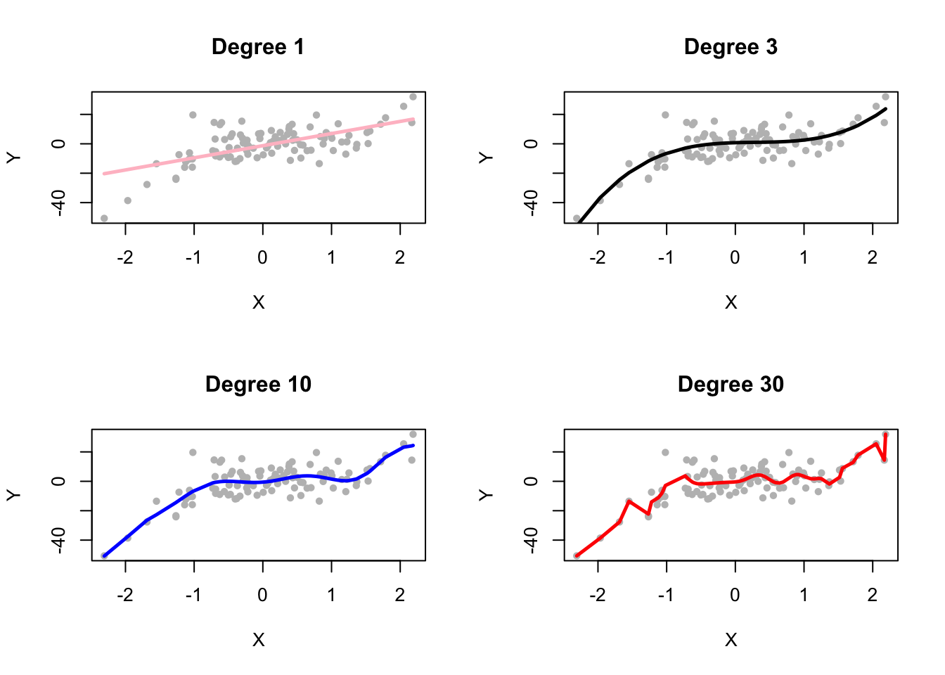
FIGURE 6.1: OLS fits for polynomial degrees 1, 3, 10, and 30
In Figure 6.1, we visualize the fits of OLS models for polynomial degrees 1, 3, 10, and 30, as applied to the generated data. Each subplot represents fit of the model for a specific degree, allowing us to compare how the complexity of the polynomial impacts the model’s ability to capture the underlying data-generating mechanism. As the degree increases, we observe how the model becomes increasingly flexible (complex), fitting the training data more closely. In particular, the degree 1 and 3 models provide smoother, simpler fits, while the degree 10 and 30 models capture more intricate patterns, and begin to overfit the noise in the data.
6.1 Out-sample MSPE
In Table 6.1 below, we compare the in-sample and out-sample Mean Squared Prediction Errors (MSPE) for polynomial degrees ranging from 1 to 10. The in-sample MSPE values, starting from 87.7267 for degree 1 and decreasing to 56.2245 for degree 10, are the exact same ones calculated in the previous chapter. In contrast, the out-sample MSPE values are newly calculated, with the lowest out-sample error occurring at degree 3 (66.1662), after which it begins to rise, reaching 71.0181 at degree 10. This behavior illustrates how, as model complexity increases, the in-sample MSPE continues to decrease as the model better fits the training data, while the out-sample MSPE initially decreases but eventually rises due to overfitting.
To select the “best” predictive model, we focus on the model with the lowest out-sample MSPE, rather than the in-sample MSPE. This is because the out-sample MSPE better reflects the ability of the model to generalize to unseen data, while the in-sample MSPE only measures how well the model fits the training data. In this case, the model with polynomial degree 3 offers the best predictive performance, as it achieves the lowest out-sample MSPE. Below, we will discuss how these out-sample MSPE values were calculated and the implications for model selection.
| Polynomial Degree | In-sample MSPE | Out-sample MSPE |
|---|---|---|
| 1 | 87.7267 | 87.7241 |
| 2 | 82.9245 | 84.2082 |
| 3 | 60.9356 | 66.1662 |
| 4 | 60.1289 | 66.9232 |
| 5 | 59.5444 | 67.6132 |
| 6 | 59.0234 | 68.4805 |
| 7 | 58.4406 | 68.9593 |
| 8 | 57.7283 | 69.5755 |
| 9 | 56.9430 | 70.3915 |
| 10 | 56.2245 | 71.0181 |
Table 6.1 presents a comparison of in-sample and out-of-sample MSPEs for polynomial degrees 1 through 10. It highlights the trade-off between model complexity and predictive performance, aligning with the U-shaped behavior illustrated in the earlier figure. The in-sample MSPE is shown in Figure 6.2 with a gray dashed line and triangle markers, while the out-sample MSPE is plotted using a black solid line and circle markers.
As the plot illustrates, the in-sample MSPE decreases steadily with increasing polynomial degree. This is expected, as more flexible models fit the training data more closely—capturing both the signal and some noise—which drives down the training error. By degree 10, the in-sample MSPE reaches its lowest point, reflecting an almost perfect fit to the training data.
In contrast, the out-sample MSPE follows a U-shaped curve. It initially decreases and reaches its minimum around degree 3, indicating that a degree 3 model best balances fit and generalization. Beyond that point, the out-sample MSPE rises again, suggesting that higher-degree models begin to overfit the training data and perform worse on unseen data.
This pattern exemplifies the bias-variance tradeoff: low-degree models are too rigid (high bias), while high-degree models become too sensitive to noise (high variance). The degree 3 polynomial offers the optimal trade-off, minimizing out-sample MSPE and yielding the best predictive performance.
Ultimately, the simulation reinforces a central principle of statistical learning: the model that minimizes out-sample error—not in-sample error—is the most reliable for prediction. Choosing the right level of complexity is key to avoiding overfitting and achieving strong generalization.
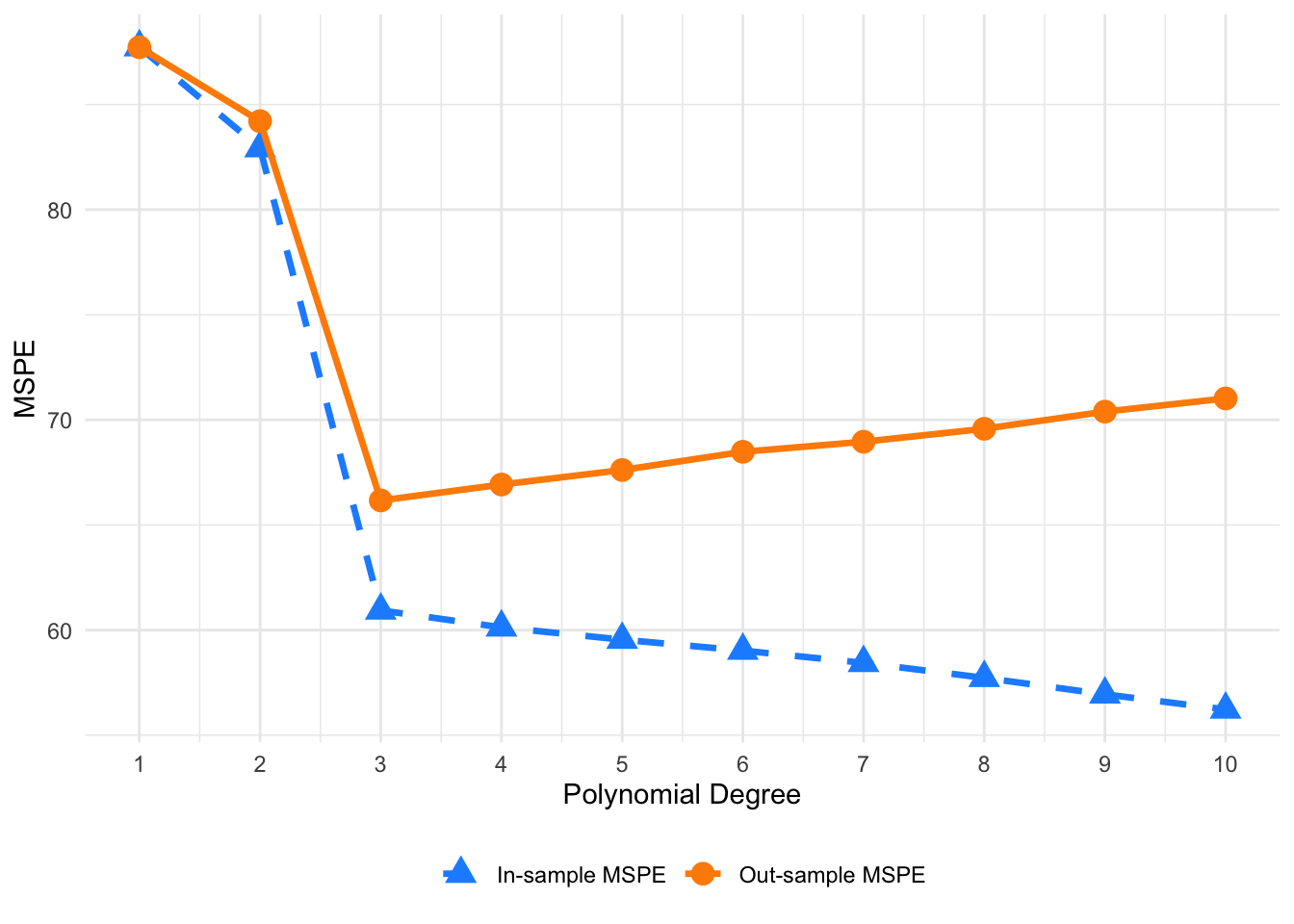
FIGURE 6.2: Comparison of in-sample and out-of-sample MSPEs across polynomial degrees
In the previous chapter, we showed in detail how to calculate in-sample MSPE as well as its components such as bias squared, variance, and irreducible error. Although the process for out-sample MSPE is very similar, there is a major difference. However, you can easily implement a similar simulation for out-sample MSPE, so we will not discuss every step in detail. Here is how out-sample MSPE is calculated, not only in this simulation but also for all real data applications.
To evaluate the generalization performance of the models, we calculate the out-sample mean squared prediction error (MSPE). For this, we use a similar approach as with the in-sample MSPE but with one key difference: instead of calculating the error on the same data, i.e., the training data, used to fit the model, we use an independent test dataset. The out-sample MSPE gives us an indication of how well the fitted models, \(\hat{f}\), generalize to new, unseen data.
In this setup, we generate 50 training datasets, \(\mathcal{D}\), with a sample size of \(n = 100\), and fit polynomial regression models of degrees ranging from 1 to 10 using ordinary least squares (OLS). These models are trained (estimate the model parameters, \(\beta\)) on the training data, and we calculate the prediction functions for each degree as follows:
\[ \hat{f}_1(x) = \hat{\beta}_0 + \hat{\beta}_1 x \]
\[ \hat{f}_2(x) = \hat{\beta}_0 + \hat{\beta}_1 x + \hat{\beta}_2 x^2 \]
\[ \hat{f}_3(x) = \hat{\beta}_0 + \hat{\beta}_1 x + \hat{\beta}_2 x^2 + \hat{\beta}_3 x^3 \]
\[ \vdots \]
\[ \hat{f}_{10}(x) = \hat{\beta}_0 + \hat{\beta}_1 x + \hat{\beta}_2 x^2 + \ldots + \hat{\beta}_{10} x^{10} \]
For each dataset, we estimate the model parameters, \(\beta\), based on the training data. These parameters are exactly the same \(\beta\)’s we estimated in the simulation used to calculate the in-sample MSPE in the previous chapter. Then, using these estimated parameters, we predict the values of \(Y\) on a separate, independent test dataset. This allows us to calculate the , which is the average squared difference between the predicted values from the model and the actual observed values in the test data.
We repeat this process for 50 training and test datasets. For each polynomial degree, we compute the expected out-sample MSPE by averaging the results across the 50 test datasets. This allows us to assess how each model performs on new data, providing a clear picture of which degree of polynomial achieves the best trade-off between bias and variance.
To conclude, understanding and managing the bias-variance tradeoff is essential in selecting a model that not only fits the training data well but also generalizes effectively to unseen data, ultimately minimizing overfitting and improving predictive accuracy. In the context of regression, selecting the right model complexity is crucial to balancing the tradeoff between bias and variance. A model is biased when it oversimplifies the relationship between the variables, such as when a linear model is used to fit a quadratic relationship. On the other hand, a model becomes too variable when it overfits the data, incorporating too many variables or allowing for excessive flexibility, such as fitting a cubic model to a linear relationship. In non-parametric models, bias occurs when too much smoothing is applied, while variance increases when the model becomes overly “wiggly” and captures noise in the data.
Throughout this chapter, we have explored how increasing model complexity affects both train MSPE and test MSPE. As model complexity grows, the train MSPE decreases, since the model fits the training data more closely. However, the test MSPE follows a U-shaped curve, decreasing at first as the model captures the underlying patterns in the data, but eventually increasing as overfitting sets in. This behavior underscores the importance of selecting a model that balances bias and variance to minimize reducible error and perform well on unseen observations.
By understanding the bias-variance tradeoff, we can fine-tune model complexity to avoid the extremes of underfitting and overfitting. Ultimately, the goal is to find the optimal point where the model is flexible enough to capture the true relationship in the data, but not so complex that it loses its ability to generalize to new data. This balance is key to building models that predict effectively and robustly.
6.2 Technical Points about Out-sample and In-sample MSPE
For Linear Regression with a Linear Population Model, we define MSPE over some data points, as we did in our simulation above, and rewrite it as follows:
\[\begin{equation} \mathbf{MSPE}_{out} = E\left[\frac{1}{n} \sum_{i=1}^{n} \left(y'_{i} - \hat{f}(x_i)\right)^{2}\right],~~~~~~\text{where}~~y'_i = f(x_i) + \varepsilon'_i \end{equation}\] This type of MSPE is also called unconditional MSPE. Inside the brackets is the “prediction error” for a range of out-of-sample data points. The only difference here is that we distinguish \(y'_i\) as out-of-sample data points. Likewise, we define MSPE for in-sample data points \(y_i\) as
\[\begin{equation} \mathbf{MSPE}_{in} = E\left[\frac{1}{n} \sum_{i=1}^{n} \left(y_i - \hat{f}(x_i)\right)^{2}\right],~~~~~~\text{where}~~y_i = f(x_i) + \varepsilon_i \end{equation}\] Note that \(\varepsilon'_i\) and \(\varepsilon_i\) are independent but identically distributed. Moreover, \(y'_i\) and \(y_i\) have the same distribution.
The relationship between the out-sample MSPE and in-sample MSPE can be expressed as:
\[\begin{equation} \mathbf{MSPE}_{out} = \mathbf{MSPE}_{in} + \frac{2}{n} \sigma^2(p+1) \end{equation}\] The last term quantifies the overfitting, which reflects how the in-sample MSPE systematically underestimates the true MSPE, i.e., the out-sample MSPE. Additionally, the overfitting
Thus, as we discussed earlier, the overfitting problem worsens as \(p/n\) becomes larger. Minimizing the in-sample MSPE completely ignores overfitting, resulting in models that are too large and have very poor out-sample prediction accuracy.
Now, let’s look closer at \(E\left[(y'_i - \hat{f}(x_i))^2\right]\). Using the definition of variance, we can express it as:
\[\begin{align} E\left[(y'_i - \hat{f}(x_i))^2\right] &= Var\left[y'_i - \hat{f}(x_i)\right] + \left(E\left[y'_i - \hat{f}(x_i)\right]\right)^2 \notag \\ &= Var\left[y'_i\right] + Var\left[\hat{f}(x_i)\right] - 2\, Cov\left[y'_i, \hat{f}(x_i)\right] + \left(E\left[y'_i\right] - E\left[\hat{f}(x_i)\right]\right)^2 \end{align}\]
Similarly, for in-sample points:
\[\begin{align} E\left[(y_i - \hat{f}(x_i))^2\right] &= Var\left[y_i - \hat{f}(x_i)\right] + \left(E\left[y_i - \hat{f}(x_i)\right]\right)^2 \notag \\ &= Var\left[y_i\right] + Var\left[\hat{f}(x_i)\right] - 2\, Cov\left[y_i, \hat{f}(x_i)\right] + \left(E\left[y_i\right] - E\left[\hat{f}(x_i)\right]\right)^2 \end{align}\]
Recall our earlier discussion on variance-bias decomposition: when predicting out-sample data points, \(y'_i\) and \(\hat{f}(x_i)\) are independent. Alternatively, \(\varepsilon'_i\) is independent of \(\hat{f}(x_i)\). In other words, how we estimate \(\hat{f}(x_i)\) is independent of \(y'_i\). Hence, \(Cov\left[y'_i, \hat{f}(x_i)\right] = 0\). However, it is important to understand that \(Cov\left[y_i, \hat{f}(x_i)\right] \neq 0\) for in-sample data. This is because \(\hat{f}(x_i)\) is chosen to minimize the difference from \(y_i\). Therefore, the estimator is not independent of in-sample points \(y_i\); rather, they are used to estimate \(\hat{f}(x_i)\). In fact, if \(\hat{f}(x_i) = y_i\), the MSPE would be zero, and the correlation between \(\hat{f}(x_i)\) and \(y_i\) would be 1.
Using the fact that \(E(y'_i) = E(y_i)\) and \(Var(y'_i) = Var(y_i)\), we can rewrite \(E\left[(y'_i - \hat{f}(x_i))^2\right]\) as:
\[\begin{align} E\left[(y'_i - \hat{f}(x_i))^2\right] &= Var[y_i] + Var[\hat{f}(x_i)] + \left(E[y_i] - E[\hat{f}(x_i)]\right)^2 \notag \\ &= E\left[(y_i - \hat{f}(x_i))^2\right] + 2\, Cov[y_i, \hat{f}(x_i)] \end{align}\]
Averaging over all data points:
\[\begin{equation} E\left[\frac{1}{n} \sum_{i=1}^{n} \left(y'_i - \hat{f}(x_i)\right)^2\right] = E\left[\frac{1}{n} \sum_{i=1}^{n} \left(y_i - \hat{f}(x_i)\right)^2\right] + \frac{2}{n} \sum_{i=1}^{n} Cov[y_i, \hat{f}(x_i)] \end{equation}\]
\[\begin{equation} \frac{2}{n} \sum_{i=1}^{n} Cov[y_i, \hat{f}(x_i)] = \frac{2}{n} \sigma^2(p+1) \end{equation}\] Thus, we arrive at the relationship:
\[\begin{equation} \mathbf{MSPE}_{out} = \mathbf{MSPE}_{in} + \frac{2}{n} \sigma^2(p+1) \end{equation}\]